About EURODL |  Sections |  Subscription |  For Authors |  Special Issues |  Archives   Peer-reviewed articles |  Brief items |  Reviews

NEW

Best of EDEN 2018 Special issue
 

There are not any recent contributions.

There are not any recent contributions.

Archives

2020/I 2019/II 2019/I 2018/II 2018/I 2017/II 2017/I 2016/II 2016/I 2015/II

2015/I 2014/II 2014/I 2013/II 2013/I 2012/II 2012/I 2011/II 2011/I 2010/II

2010/I 2009/II 2009/I 2008/II 2008/I 2007/II 2007/I 2006/II 2006/I 2005/II

2005/I 2004/II 2004/I 2002 2001 2000 1999 1998 1997

EURODL Mailinglist

2851 subcribers
 

EURODL Visitors

back

Adaptive Competence Testing in eLearning

Gisela Dösinger, Dietrich Albert
Know-Center Graz, Universität Graz, Austria

Key words: Adaptive testing, assessment algorithm, competence-performance approach, eLearning, knowledge modelling, personalisation

Abstract:

This article focuses on the adaptive assessment of pre-knowledge in the context of individualised eLearning. A deterministic algorithm [3] is introduced which allows for a significant reduction of to be presented problems for diagnosing pre-knowledge. Since the competence-performance approach [12] , [13] , [14] is used for building the framework for adaptive testing, not only can it efficiently be assessed which problems a learner is able to master, but also which knowledge, abilities, and skills are available. Such an adaptive competence assessment is of importance when learning units for individualised  instruction have to be chosen by a learning program. The algorithm, the competence-performance approach, and a practical example, next to a foresight concerning the planning of testing procedures are introduced in this article.

1         Introduction

Individualisation is of increasing importance with respect to eLearning. Even though not well established yet in the domain of technology-based training, the concept of individualisation or personalisation, respectively, denotes a general educational principle to which traditional instruction obeys. The term stands for the individualisation of training as well as of content to various characteristics of the learner. It requires instruction to meet the current learning level, rate of learning, cognitive and learning style, contexts known to the learner, previous experiences, feelings, needs and interests. While a human teacher easily, intuitively and in a flexible manner is able to adapt to the individual learner in these concerns, personalisation is a much more complex task within eLearning. Not only have the technological foundations to be developed, but also have the aspects in which individualisation is possible to be identified, precisely described, and systematised. Only then they can be implemented in a rule-driven way so that flexible learning programs can be developed.

In this article, concerning individualisation, we will concentrate on the diagnosis of pre-knowledge in terms of competencies that are required for the solution of problems. The assessment of pre-knowledge is important for optimally adapting lessons to the learner in the sense that he is only taught what he does not know yet and not bored with known contents. By diagnosing the knowledge already available in a given domain it is prevented that the learner either is unchallenged or that there is demanded too much from him. This in turn supports the motivation to learn and saves concentration for the relevant contents. Of course, the assessment should be efficient, not demanding too much time and cognitive resources.

Since only human teachers can - by using their implicit knowledge - intuitively and flexibly adapt to their pupils, in the case of technology-based training a systematics is required according to which the learning level can efficiently be assessed and, based on it, further instruction can be planned. Such a systematic is provided by a competence-performance approach developed by Korossy [12] , [13] , [14] , [15] which is an extension of knowledge space theory [2] , [6] . By its means not only adaptive and hence efficient testing becomes possible but also does it allow for organising learning processes. This approach makes use of solution dependencies among problems which are based on their qualitative description, that is, on the assignment of knowledge entities explaining their solution.

In the following the theoretical foundations of the above mentioned approach will be introduced as well as practical examples demonstrating its applicability will be reported. In this context a deterministic algorithm [3] allowing for the efficient diagnosis of knowledge by means of the observable solution behaviour of a learner will be introduced.

2         Modelling a knowledge domain

2.1        Theoretical foundations

The foundation of an adaptive instrument which at the same time serves as the framework for a curriculum consists in an order - a not necessarily linear order - on a set of problems. The solution dependencies among the problems, which define the order, are of the kind that from the solution of a super ordinate problem the solution of a subordinate problem can be derived without actually observing the solution of the latter one.

For developing computerised adaptive tests item response theory [7] is generally used. Next to not allowing for non-linear orders on a set of problems, its greatest disadvantage is that on its basis competence assessment is not possible, in the sense, that all the competencies contributing to the solution of a problem are diagnosed and not just an overall ability. It can only be determined which problems a learner is able to master and to what extent an overall ability underlying the solution of problems is available, but not which knowledge entities in particular had been applied for solving the problems because it is not made explicit which knowledge entities contribute to the solution of each problem. To meet these problems we suggest a competence-performance approach [12] , [13] , [14] as an alternative for constructing adaptive tests. It systematically relates problems and knowledge required for solution to each other so that from the observed solution behaviour the inference to the underlying knowledge can be drawn, that is, competence assessment becomes possible. Explicitly differentiating between a latent and a manifest level of knowledge, that is competence and performance, and connecting these levels to each other can be said to be the key concept of this approach. Performance stands for the observable solution behaviour – a subject masters a problem or it fails - while competence stands for the underlying knowledge, abilities, and skills explaining the performance. The competence-performance approach is an extension of the knowledge space theory [2] , [6] .

In the following the steps for establishing an order on a set of problems, that is, for developing a model according to the competence-performance approach, are briefly outlined in a formal way.

Step 1: Identifying and representing solution paths

Let there be a set Q of problems q and a set E of elementary competencies e - abilities and skills - representing a knowledge domain W.

As a first step it is analysed which solution paths there exist for arriving at the solution of a problem, that is, it is analysed how a problem can be solved. For each problem there may be more than one solution path. Next, the distinct steps into which the solution paths can be split up are described by the elementary competencies. Problems and elementary competencies required for solving the problems are mapped to each other by the function f: Q®Ã(Ã(E)) [1] . The subsets assigned to the problems are summarised in the set L=È{ f (Q)|qÎQ}.

Step 2: Obtaining the competence space

By closing the set L under union the competence structure K is obtained. If for all the problems there has been assigned only one solution path the competence structure is said to be a quasi ordinal competence space which is stable under union and intersection. If there exist alternative solution paths the resulting knowledge structure is said to be a competence space which is only stable under union. The subsets of elementary competencies obtained by the closure under union are called the competence states k. They are elements of the competence structure.

Step 3: Relating the levels of competence and performance to each other

In a next step the interpretation function k: Q®Ã(K) is applied. It assigns all those competence states to each problem in which it is solvable. A problem is solvable in a certain state when the state assigned to it by the function f is a subset of the viewed state. The interpretation function induces the representation function p: K ®Ã(Q). It assigns all those problems to each of the competence states that are solvable in it. A problem is solvable in a certain competence state when the state as assigned to it by the function f is a subset of the viewed state. The subsets of problems as assigned to each competence state by the representation function are called performance states p(k). They are element of the performance structure P. A quasi ordinal performance space results if only one solution path had been identified for each problem. With exceptions, in general, a performance space results if more than one solution path had been assigned to a problem.

Step 4: Deriving the order on the set of problems

From the performance structure the solution dependencies among the problems can be read. They are obtained by first assigning all the performance states p(k)_q to each problem q that contain it and by then extracting those performance states per problem that are minimal concerning the subset relation Í. The solution dependencies are represented by a so called surmise relation ≼ or surmise system s in the case of a quasi ordinal performance space or performance space, respectively. Graphically the order on the set of problems can be depicted in an upward-drawing or an and/or-graph, respectively. For each two problems that are related to each other it holds that if the super ordinate problem is solved the solution of the sub-ordinate can be surmised.

2.2        A practical example

For demonstrating the applicability and usefulness of the discussed methodology the domain W of counting competence in preschoolers was chosen. It is represented by a problem set Q={q₁,q₂,q₃,q₄,q₅} and a set of elementary competencies E={e₁,e₂,e₃,e₄,e₅} accounting for the solution of the problems [2] . For a brief description of the problems and elementary competencies see the appendix.

In the following the single steps of modelling as introduced in a formal way in the previous section are explained by means of the example. Here, we consider only the case of one solution path per problem. In this case it can uniquely be determined which knowledge the learner has available.

Step 1: Identifying and representing solution paths

The solution paths are not verbally described here but are reported by means of the representing subsets of elementary competencies that account for the solution of the problems. The function f which assigns exactly these subsets to problems is displayed in table 1. The subsets f(q) are summarised in the set L.

Table 1

Function f assigning problems to subsets of elementary competencies sufficient for solving the problems

L={{e₁},{e₁,e₂},{e₁,e₂,e₃},{e₁,e₂,e₄},{e₁,e₂,e₄,e₅}}

Step 2: Obtaining the competence space

By closing the set L under union a quasi-ordinal competence space K is obtained. Since per definition the competence space always contains the empty set it consists of 8 competence states k.

K ={{},{e₁},{e₁,e₂},{e₁,e₂,e₃},{e₁,e₂,e₄},{e₁,e₂,e₄,e₅},{e₁,e₂,e₃,e₄},{e₁,e₂,e₃,e₄,e₅}}

Step 3: Relating the levels of competence and performance to each other

In a next step, first, the interpretation function k: A®Ã(K) is applied. It assigns all those competence states to each problem which account for its solution. Second, through the representation function p: K ®Ã(Q) all those problems are assigned to each competence state which can be solved in it. Table 2 displays both functions at once.

For an explanation of the interpretation function k consider row four. Problem q₃ is mapped to three competence states. One of these is the state {e₁,e₂,e₃} as assigned by the function f - indicated by ¨ - and the others {e₁,e₂,e₃,e₄} and {e₁,e₂,e₃,e₄,e₅} - they are indicated by a · - are those which the first is a subset of. All these states allow for solving the problem.

For an explanation of the representation function p consider column six. All the problems are mapped to the competence state {e₁,e₂,e₄} which are solvable in it. The problems can be said to be solvable in that state because the states {e₁},{e₁,e₂} and {e₁,e₂,e₄} which are sufficient for their solution are subsets of it.

Table 2

Interpretation function k and representation function p

	{}	{e1}	{e1,e2}	{e1,e2,e3}	{e1,e2,e4}	{e1,e2,e4,e5}	{e1,e2,e3,e4}	{e1,e2,e3,e4,e5}
q1		¨	·	·	·	·	·	·
q2			¨	·	·	·	·	·
q3				¨			·	·
q4					¨	·	·	·
q5						¨		·
	{}	{q1}	{q1,q2}	{q1,q2,q3}	{q1,q2,q4}	{q1,q2,q4,q5}	{q1,q2,q3,q4}	{q1,q2,q3,q4,q5}

The subsets of problems as assigned by the representation function are given in the bottom row of table 2. They constitute the performance space

P ={{},{q₁},{q₁,q₂},{q₁,q₂,q₃},{q₁,q₂,q₄},{q₁,q₂,q₄,q₅},{q₁,q₂,q₃,q₄},{q₁,q₂,q₃,q₄,q₅}}.

Step 4: Deriving the order on the set of problems

From the performance space the dependencies among the problems and hence the order on the set of problems can be read. First, all those performance states p(k)_q are assigned to each problem q that contain it. Then, these performance states are extracted per problem that are minimal concerning the subset relation Í. Table 3 displays the procedure. The minimal states are indicated by bold letters.

Table 3

Determining solution dependencies

The resulting dependencies among the problems are graphically depicted in the form of an upward-drawing in figure 1. The solution of all the problems which are reached by a descending line starting at one problem can be surmised from this problem.

Figure 1

Upward drawing depicting the dependencies among the problems

Before a structure can be used for the individualised diagnosis of knowledge it has to be empirically validated first. Only if it is valid the obtained order on the set of problems can be used for adaptive testing. Since it is not the purpose of this paper to present validation methods the standard method will only briefly be described.

For the validation of the obtained structure the problems have to be presented to a number of subjects. For each subject it has to be assessed which problems it is able to solve and which not. The subset of solved problems is called a solution pattern X. For each solution pattern it is determined to which degree it corresponds to the hypothesised structure on the set of problems. This is done by calculating the symmetric distance between each solution pattern X and each performance state p(k). The symmetric distance d is defined as the number of problems contained in either set but not the other, in general d(M,N)=|MDN|=|M\N|È|N\M|. For each solution pattern distances varying between zero - indicating a perfect fit - and the maximal possible distance Q/2 - indicating worst fit - is obtained. The minimal observed distance per solution pattern is taken for calculating the average distance which provides information about the overall model fit. In general, the smaller the observed distance the better the fit. Of course, some more measures exist for deciding about the validity of the model. This measures should only be mentioned: Gamma-Index [8] ,[16] , Distance Agreement Coefficient [17] , Reproducibility Coefficient [9] .

Concerning our example the fit of the model was sufficiently high so that the structure can be used as the basis for adaptive testing.

In the following it is described how in an adaptive testing procedure based on a deterministic algorithm [3] problems are chosen for presentation and how thereby the number of to be presented problems can be reduced compared to a conventional assessment. The underlying principle of the algorithm working on the performance space is introduced in the following section.

3         A deterministic algorithm for adaptive testing

In this section a deterministic algorithm which works on the basis of a binary search method is introduced [3] . In the following it is described how dependent on the solution behaviour by means of the algorithm it is decided upon the problems for presentation.

The first to be presented problem is chosen in a way so that it divides the performance space into two subsets containing nearly the same number of performance states: one subset consisting of performance states containing the viewed problem and the other subset not containing it. If the presented problem is not solved all the states containing it can be cancelled concerning the ongoing questioning procedure. The next problem then is chosen from the remaining performance states, again in a way, so that they are divided in two subsets containing nearly the same number of performance states. If, on the contrary, the problem is solved the next to be presented problem in the same way is chosen from the set of performance states that contain it. The states not containing it are cancelled. The algorithm repeatedly applies as long as no definite conclusion about the expected mastery of problems can be drawn on the basis of solution dependencies.

For demonstrating how the algorithm works let us refer to our example. Two exemplar knowledge diagnoses are described in the following. Figure 2 supports their verbal description.

In both diagnoses the problem that is chosen to be presented first is problem q₃ because it divides the performance space into two subsets containing nearly the same number of performance states. The subsets consist of the performance states which do and which do not contain problem q₃ respectively.

In diagnosis 1 problem q₃ is mastered. Next, problem q₅ is chosen for presentation because it divides the set of states containing problem q₃ into two subsets containing nearly the same number of performance states, consisting of the performance states which do and which do not contain problem q₅, respectively. Problem q₅ is again mastered. Thus, dependent on the relationships among the problems we can conclude that the subject who mastered problems q₅ and q₃ is in the performance state {q₁,q₂,q₃,q₄,q₅}. Since the problems were described by the competencies required for their solution, by examining which problems a subject is able to master, the underlying knowledge can uniquely be assessed. The competence diagnosis is of great importance because based on it further instruction can be planned. As can be read from table 2 the performance state {q₁,q₂,q₃,q₄,q₅} arises from the competence state {e₁,e₂,e₃,e₄,e₅}.

In diagnosis 2 problem q₃ is not mastered. Thus, the subject cannot be in any state that contains problem q₃. Therefore, from the set of states not containing problem q₃ problem q₄ is chosen next because it divides the set into two subsets containing nearly the same number of performance states, consisting of the performance states which do and which do not contain problem q₄ respectively. The subject fails on problem q₄. So, the states containing it are cancelled while from the remaining states not containing it problem q₂ is chosen because it divides these states into halves that are nearly equal concerning the number of states. Since the subject solves problem q₂ no further problem has to be presented. We can conclude that the subject is in the state {q₁,q₂}. Since we are interested in the knowledge which explains the solution of the problems we look at the corresponding competence state. From table 2 it can be read that someone who is able to master problems q₁ and q₂ has available the competencies e₁ and e₂. The competencies e₃ through e₅ the learner has still to be taught.

The two exemplar diagnoses show that actually savings are reached by making use of the introduced algorithm working on the performance space. Instead of five problems only two and three respectively had to be presented for uniquely determining which problems the learner is able to master and, what is more important, which competencies the learner had available. In general, the proportion of problems which can be saved depends on the kind of order. Savings will be the higher, the more pairs are in the relation.

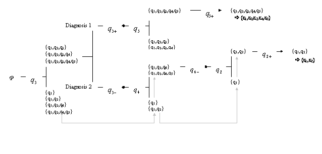
Figure 2

Graphical depiction of two exemplar diagnoses based on a deterministic algorithm

Note. + …problem is solved, - …problem is not solved.

4         Fuzzy competence assessment

While in the previous section the case of one solution path per problem had been considered, here the more realistic case of more than one solution path per problem is introduced. As it was said earlier, in the latter case a unique competence assessment is no longer possible. If alternative solution paths exist the number of competence states characterising the knowledge of a subject does not equal one but can only be equated with a number of possible competence states each sufficient to explain the observable solution behaviour. These competence states are summarised in so called competence classes. Thus, competence assessment remains fuzzy [15] .

For introducing the fuzzy assessment as a result of alternative solution paths an example concerning numerical and prenumerical reasoning in preschool age was constructed [3] . Consider a problem set Q={r₁,r₂,r₃} and a set of elementary competencies E={b₁,b₂,b₃} accounting for the solution of the problems. For a brief description of the problems and elementary competencies see the appendix. As in the first example the single steps of modelling are worked out.

Step 1: Identifying and representing solution paths

Again, the solution paths are not verbally described here but are reported by means of the representing subsets of elementary competencies as obtained by the competence analysis. As can be seen in table 4 problems r₁ and r₂ require the competencies b₁ or b₂ for solution. The same is true for problem r₃: the competence states {b₁,b₃} or {b₂,b₃} explain its solution. The function f assigning exactly these subsets to the problems is displayed in table 4. The subsets f(q) are summarised in the set L.

Table 4

Function f assigning problems to subsets of elementary competencies sufficient for solving the problems

L={{b₁},{b₂},{b₁,b₃},{b₂,b₃}}

Step 2: Obtaining the competence space

By closing the set L under union the competence space K is obtained. It contains 7  competence states k.

K ={{},{b₁},{b₂},{b₁,b₂},{b₁,b₃},{b₂,b₃},{b₁,b₂,b₃}}

Step 3: Relating the levels of competence and performance to each other

Next, the interpretation function k: A®Ã(K) and the representation function p: K®Ã(Q)  which is induced by the first are applied. Table 5 displays both functions at once. For an explanation of the functions and table 5 see section 2.

Table 5

Interpretation function k and representation function p

The subsets of problems as assigned by the representation function are given in the bottom row of table 5. They constitute the performance space

P ={{},{r₁,r₂},{r₁,r₂,r₃}}.

Step 4: Deriving the order on the set of problems

From the performance space the dependencies among the problems and hence the order on the set of problems can be read. According to the procedure as introduced in section 2.1 the dependencies among the problems are determined: problem r₃ presupposes problems r₁ and r₂, that is, from the solution of problem r₃ the solution of problems r₁ and r₂ can be surmised. This dependency is graphically depicted in an upward-drawing in figure 3.

q1

r3

{r1,r2}

Figure 3

Upward-drawing depicting the dependencies among the problems

Due to the simplicity of this example it can easily be seen what we intend to point out. As the top and bottom row of table 5 show, there are different competence states which give rise to the same performance states. Thus, from the observed performance it can no longer uniquely be derived which competencies in particular the learner has available, only the competence class can be determined. If we observe a subject mastering r₁ and r₂ we cannot say clear-cut whether the subject has available competency b₁ or b₂ or both. The same is true when a learner is observed mastering problems r₁, r₂ and r₃. Either the learner has available competencies b₁ and b₃ or b₂ and b₃ or b₁, b₂, and b₃. Thus, the competence assessment remains fuzzy. But this ambiguity can be dissolved. If in the assessment procedure we land at such a situation we simply need to construct a further problem which concerning the competencies the learner has available is informative. In the example at hand we could e.g. construct a problem which can only be solved if both competencies b₁ and b₂ are available. If the subject is able to solve this problem it can uniquely be determined that the subject has available both competencies. Of course, the competence assessment can only be made precise at cost of a higher number of to be presented problems. But, nevertheless adaptive assessment remains possible and additional problems need only be suggested by a learning program if such a situation is met.

5         Conclusion

In the following it will be discussed in which concerns the above introduced methodology can be made use of.

In the domain of performance testing - final exams, recruitment tests, college admission test - it is of importance to have a large pool of problems from which the problems can randomly be chosen so that from test to test different problems are presented. The presentation of different problems is of importance because it has to be prevented that the to be tested persons prepare for the tests and learn the responses. If persons are prepared the tester cannot get an impression of the true ability of the tested person. To get parallel, that is, comparable tests which still test the same knowledge and allow for a comparison of the tested persons the problems of an existing test have to be analysed for their requirements first. Then, on their basis problems can be constructed that require just the same combinations of competencies for solution as their antetypes. After thereby a large pool of problems has been generated for different samples of to be tested persons in an automatic way different tests can be composed.

So far, the application of the competence-performance approach has only been discussed in the domain of testing. But it can also be used for organising learning processes [15] , concerning eLearning, for an online curriculum generation on an individual level. If the competence and the performance space are implemented into a learning program, first the current competence level can be assessed - it does not matter whether the competence assessment is precise or fuzzy -  and based on it the learner can be taught those competencies which he does not have available yet, but which he is most disposed to learn. That is, the learner is taught exactly these competencies in which the super-ordinate problem not yet solved differs from the sub-ordinate problem just solved. Some adaptive tutoring systems based on knowledge space theory - even though not on the competence-performance approach itself - already exist: AdAsTra [5] , ALEKS [3] , and RATH [10] , [11] , [1] .

A still open issue concerns the application of the competence-performance approach to more self-directed learning situations which lack structure. At first sight unstructured learning situations may contradict the assessment of knowledge in terms of the competence-performance approach. But in our opinion also here it can reasonably be applied. Consider learning units not connected to each other in the sense of dependencies among problems as the are defined according to the competence-performance approach, but sufficiently be described by underlying competencies. If any combination of the underlying competencies is represented by a problem, a structure on the set of problems can be derived. After the learner has worked on an arbitrary set of units, the corresponding substructure of problems can be taken out from the overall structure. Then it can adaptively be assessed which problems a student is able to master and hence which competencies he has available and is able to apply in combination. On this basis, it can be determined which competencies the learner has still to be taught. Moreover, it can be concluded for which competencies a joint application is not yet possible. This procedure prevents that entire learning units have to be repeated. Instruction can focus on the teaching of single competencies and on helping the learner to integrate competencies for their joint application.

Acknowledgements

The Know-Center is a Competence Center funded within the Austrian K plus Competence Centers Program (www.kplus.at) under the auspices of the Austrian Ministry of Transport, Innovation and Technology.

References:

[1]     Albert, D. & Hockemeyer, C. (1997). Adaptive and dynamic hypertext tutoring systems based on knowledge space theory. In B. du Boulay & R. Mizoguchi (Eds.), Artificial Intelligence in Education: Knowledge and Media in Learning Systems, (pp. 553-555). Amsterdam: IOS Press.

[2]     Doignon, J.P. & Falmagne, J.C. (1985). Spaces for the assessment of knowledge. International Journal of Man-Machine Studies, 23, 175-196.

[3]     Doignon, J.P. & Falmagne, J.C. (1999). Knowledge Spaces. Berlin – Heidelberg – New York : Springer Verlag.

[4]     Dösinger, G. (2002). Conceptions and misconceptions in the domain of early mathematics. An empirical approach based on the theory of knowledge spaces and information systems. Unpublished manuscript, University of Graz , Austria .

[5]     Dowling, C.E., Hockemeyer, C., & Ludwig, A.H. (1996). Adaptive assessment and training using the neighbourhood of knowledge states. In C. Frasson, G. Gauthier, & A. Lesgold (Eds.), Intelligent Tutoring Systems (pp. 578-586). Berlin : Springer.

[6]     Falmagne, J.C., Doignon, J.P., Koppen, M., Villano, M. & Johannesen, L. (1990). Introduction to Knowledge Spaces: How to Build, Test, and Search Them. Psychological Review, 97(2), 201-224.

[7]     Fischer, G.H. (1995). Rasch models: foundations, recent developments, and applications. New York . Springer.

[8]     Goodman, L.A. & Kruskal, W.H. (1954). Measures of association for cross classifications. Journal of the American Statistical Association, 49, 732-764.

[9]     Guttman, L. (1944). A basis for scaling qualitative data. American Sociological Review, 9, 139-150.

[10] Hockemeyer, C. (1997b). RATH - A Relational Adaptive Tutoring Hypertext WWW-Environment. Technical report 1997/3. Graz, Austria: Institut für Psychologie, Karl-Franzens-Universität Graz.

[11] Hockemeyer, C., Held, T., & Albert, D. (1998). RATH - a relational adaptive tutoring hypertext WWW--environment based on knowledge space theory. In C. Alvegård (Ed.), CALISCE`98: Proceedings of the Fourth International Conference on Computer Aided Learning in Science and Engineering (pp. 417-423). Göteborg , Sweden : Chalmers University of Technology.

[12] Korossy, K. (1993). Modellierung von Wissen als Kompetenz und Performanz. Inauguraldisseration, University of Heidelberg .

[13] Korossy, K. (1996). Kompetenz und Performanz beim Lösen von Geometrie-Aufgaben. Zeitschrift für Experimentelle Psychologie, 43(2), 279-318.

[14] Korossy, K. (1997). Extending the Theory of Knowledge Spaces: A Competence-Performance Approach. Zeitschrift für Psychologie, 205, 53-82.

[15] Korossy, K. (1999). Organizing and Controlling Learning Processes Within Competence-Performance Structures. In D. Albert & J. Lukas (Eds.), Knowledge spaces: theories, empirical research, and applications (pp. 157-177). Mahwah , NJ : Lawrence Erlbaum Associates, Inc.

[16] Scheiblechner, H. (1999). Nonparametric IRT: Testing the bi-isotonicity of isotonic probabilistic models (ISOP). Manuscript, Philipps University Marburg .

[17] Schrepp, M. (1993). Über die Beziehung zwischen kognitiven Prozessen und Wissensräumen beim Problemlösen. Unpublished doctoral dissertation, University of Heidelberg , Germany .

Authors:

Gisela, Dösinger, Mag.
Know-Center Graz, Knowledge organisation & Knowledge Transfer
Inffeldgasse 16c, 8010 Graz
gdoes@know-center.at

Dietrich, Albert, Dr.
Universität Graz, Institut für Psychologie, Abteilung für Allgemeine Psychologie
Universitätsplatz 2, 8010 Graz
dietrich.albert@uni-graz.at

Appendix

1. Description of the problems and elementary competencies as used in the first example.

2. Description of the problems and elementary competencies as used in the second example.

---

[1] Ã…power set

[2] The example is an excerpt of the PhD-studies of the first author [4] .

[3] The PhD-studies of the first author [4] build the basis for the construction of this example.